
Naive Bayes methods are a set of supervised learning algorithms based on applying Bayes' theorem. It's actually fairly intuitive and simple to compute. Instead of looking for $p(y\mid x)$ (probability of the label, given the data) directly like discriminative models, we calculate $p(y)$ (probability of the label) and $p(x\mid y)$ (probability of the data, given the label) to find $p(y\mid x)$. This is known as a generative model. The *naive *part comes from the naive assumption that all data features are conditionally independent.
Let's say you're playing the party game Mafia. Mafia is played like this: There is one narrator/judge of the game. At the beginning, the narrator hands out cards that secretly assigns every player a role affiliated with one of three teams: Mafia, Doctors, Townspeople. The game has two alternating phases. The first is night, when everyone puts their heads down, and the narrator asks the Mafia to put their heads up, point at who they want to covertly murder, and then put their heads back down, and then repeats this process with the Doctors, having them point at who they want to save (without knowing if that person was in any danger). The second phase is day, when the narrator has everyone put their heads up, tells them who is murdered (eliminated from the game), and if that murdered person was saved by the doctors. The players then debate the identity of the mafia and vote to eliminate a suspect. Play continues until all of the mafia have been eliminated or until the mafia outnumber the doctors and townspeople.
Someone on your team has been murdered and it's on you to discover who did it. At the beginning, the narrator tells you how many people are assigned the role of Mafia, Doctor, and Townsperson. So, initially, you assign a probability to each of the survivors being mafia or innocent.
Next you start studying the features of each of the remaining survivors. Are they trying to hold in a laugh? Are they trying to avoid eye contact? Are they sweating? Are their feet pointed away from you? For each of those features, you know (subconsciously from your years of observing people) the increase or decrease in probability of the person being mafia/innocent.
For example, if the proportion of Mafia that have hair is the same as the proportion of innocent people with hair, then observing that someone has hair should not affect their probability of being mafia at all. However, if you observed that people who sweat are usually guilty, then observing someone is sweating should increase their probability of being mafia!
You can continue this as long as you want, including more and more features, each of which will modify your total probability of someone being mafia by either increasing it (if you know this particular feature is more representative of a criminal) or decreasing (if the features is more representative of an innocent person). With this data, you guess what role someone is by whether they have a higher probability of being mafia or innocent.
The benefit of such an approach is that it is rather intuitive and simple to compute. The drawback is that it assumes all features are conditionally independent. It may very well be the case that while the features isn't extremely talkative right now and is usually a loud talker on its own has close to no effect, a combination of the two (is usually a loud talker, but isn't extremely talkative right now) would actually increase the probability of someone being a mafia by a ton. This would not happen when you simply add the separate feature contributions, as described above.
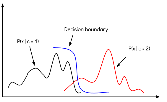
In discriminative models, you're trying to predict the most likely label $y$ from training example $x$ by evaluating $f(x) = argmax_y p(y \mid x)$ which is like modeling the decision boundary between classes.
Naive Bayes is a generative model. Instead of evaluating the conditional probability distribution $p(y \mid x)$ directly, in generative models you model the joint probability distribution $p(x, y)$, which explicitly models the actual distribution of each class.
So, with the joint probability distribution function, given a $y$, you can calculate (generate) its respective $x$. When you want to classify a new example, you can simply compare it to each of the generated class models and predict the label that it's most similar to.
Before going over Naive Bayes, first want to make sure we cover Bayes rule. Recall that, $$p(A\mid B) = \frac{p(A \wedge B)}{p(B)}$$
By using basic algebra, we can rearrange and obtain:
$$p(A\mid B) p(B) = p(A \wedge B)$$
which can also be written as:
$$p(B\mid A) p(A) = p(A \wedge B)$$
For more information on Bayes Rule, click here.
To be clear on notation:
Another form of the posterior can be written as:
$$p(A\mid B) = \frac{p(B\mid A) p(A)}{p(B\mid A) p(A)+p(B|\sim A) p(\sim A)}$$
Make sure you understand the math from above. We want to find the posterior by calculating the prior and the likelihood.
Given training data $(x_1,y_1), \dots (x_n, y_n) $ where $x_i \in \mathbb{R}$ and $y_i \in \mathbb{Y}$, your task is to learn a classification function: $f: \mathbb{R}^d \rightarrow \mathbb{Y}$.
You're basically learning a mapping $x$ to $y$ using $p(y\mid x)$. You do this by calculating the same things you would for Bayes Rule $p(y\mid x)=\frac{p(x\mid y) p(y)}{p(x)}$. You then return the class with the highest probability with:
$$argmax_y p(y\mid x)=argmax_y \frac{p(x\mid y) p(y)}{p(x)}$$
which is the same as:
$$argmax_y p(y\mid x)=argmax_y p(x\mid y) p(y)$$
As you can see, it calculates the final probability (the posterior distribution) based on the prior probability and the likelihood of the classifier.
The prior probability is simply our prior beliefs. It shows the probability of each class based on our data. If there is only 1 mafia out of 100 people, then we are always going to assume there is a smaller chance that a suspecting person is mafia.
The likelihood of the classifier is the likelihood of some (observed) data, given the labels. If you maximize the likelihood, that means you observed $x$ and want to estimate the $y$ that gave rise to it. In other words, the $y$ that maximizes $p(x\mid y)$.
This allows you to carry out Bayes rule to calculate the posterior which is the combination of the prior probability and the likelihood. You are able to calculate the probability of a new data point belonging to each class. The highest probability is the class the new data point will be classified as.
The model is simple and highly practical. This strong method is comparable to decision trees and neural networks in some cases. But why is it called naive? It's naive because it makes a strong independence assumption that's not realistic.
Consider this: we have a new example $x_{new}=(a_1,a_2, \dots, a_d)$ where $a_1, a_2, \ldots, a_d$ are the feature values and we want to predict the label $y_{new}$ of this new example.
So with Bayes, we have:
$$y_{new} = argmax_{y} p(y\mid a_1,a_2, \dots, a_d) = argmax_{y} \frac{p(a_1,a_2,\dots, a_d\mid y) p(y)}{p(a_1, a_2, \dots, a_d)}$$
which is the same as:
$$y_{new}=argmax_{y} p(a_1,a_2,\dots, a_d|y) p(y)$$
Can we estimate the two terms needed to compute Bayes from the training data? $p(y)$ can be easy to estimate: we just count the frequency of each label $y$. $p(a_1,a_2, \dots, a_d\mid y)$ however, is not easy unless we have an extremely large sample. We would need to see every example many times to get reliable estimates and finding the exact combination is hard.
So instead, we make a simplyfying assumption that the features are conditionally independent given the label. Instead of trying to find the probability that $a_1, a_2, \ldots, a_d$ all happen together given the label, we find the probability of them individually happening, given the label. So, given the label of the example, the probability of observing the conjunction $a_1, a_2, \dots, a_d$ is the product of the possibilities for the individual features:
$$p(a_1, a_2, \ldots, a_d\mid y) = \prod_j p(a_j\mid y)$$
So to predict, we have $y_{new} = argmax_{y} p(y) \prod_j p(a_j\mid y)$
Can we estimate the two terms form training data now? Absolutely!
A simple way to think about it is, prior to the naive assumption, if you see a new person in mafia that you want to predict, you have to have seen his exact features previously. For example, if the new person's features were asian, bald, tall, calm, sweating, looks innocent, and wearing a sweater, then in order to execute your calculations, you'd have to see someone with the exact features before. When we apply the naive assumption, we can assume they are all conditionally independent and can simply calculate each separate and multiply.
Given a training set ${(x_1, y_1), \ldots (x_n, y_n)}$ with $d$ features, the algorithm for Naive Bayes works like this:
You're playing mafia with 1000 people. 500 townspeople, 300 mafia, and 200 doctors. Each person has 3 features all based on your observation: whether someone looks innocent, looks helpful, *and *acts strange.
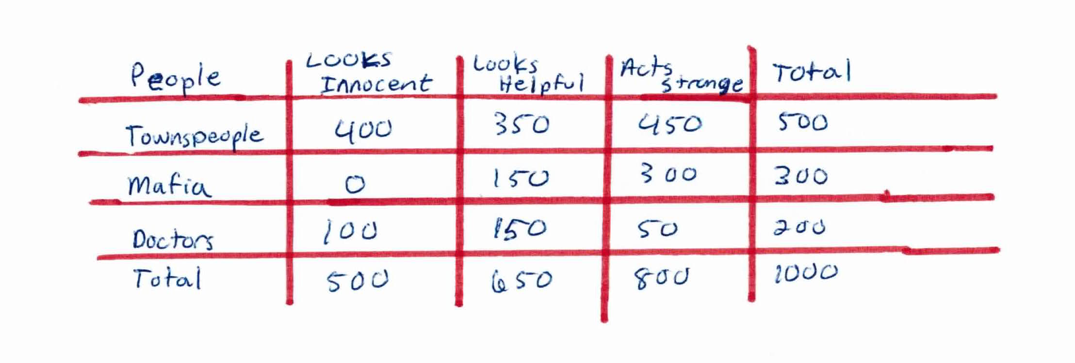
From the data above, what do we already know?
Based on our training set we can also say the following:
This data should provide enough evidence to predict whether a new person is a townsperson, doctor, or mafia.
So let’s say you start a new game of mafia. You look at the person next to you and see that they look innocent and helpful, but still act strangely. With these features you can then use your model from the previous data to predict what type of person you are facing.
$$P(T\mid I, H, S)$$
$$=\frac{P(I\mid T) P(H\mid T) P(S\mid T) P(T)}{P(I) P(H) P(S)}$$
$$= \frac{(0.8)(0.7)(0.9)(0.5)}{P(I) P(H) P(S)}$$
$$= \frac{(0.252)}{P(I) P(H) P(S)}$$
$$P(M\mid I, H, S)=0$$ (Since no mafia from your model ever looked innocent, $P(I\mid M) = 0$ causing the whole equation to be 0.)
$$P(D\mid I, H, S)$$
$$= \frac{P(I\mid D) P(H\mid D) P(S\mid D) P(D)}{P(I) P(H) P(S)}$$
$$=\frac{(0.5)(0.75)(0.25)(0.2)}{P(I) P(H) P(S)}$$
$$=\frac{(0.01875)}{P(I) P(H) P(S)}$$
Based on these calculations, we can assume that the innocent, helpful, and strange looking person is in fact a townsperson.
Naive Bayes is implemented by applying Bayes' theorem with strong (naive) independence assumptions between the features. You simply build a model for what positive examples and negative examples look like. To predict a model you use Bayes' theorem and compare the example to each model and see which one matches the best.
It is highly scalable, requiring a number of parameters linear in the number of variables (features/predictors) in a learning problem. Maximum-likelihood training can be done by evaluating a closed-form expression, which takes linear time, rather then by expensive iterative approximation as used for many other types of classifiers.
Other observations: