Logistic regression, despite its name, is a linear model for classification rather than regression. Logistic regression is a supervised classification algorithm where the dependent variable $y$ (label) is categorical, i.e. yes or no. It takes a linear combination of features with weights (parameters) and feeds it though a nonlinear squeezing function (sigmoid) that returns a probability between 0-1 of which class it belongs to. We learn the model, finding the proper weights, by using gradient descent. Those newfound weights will then be able to classify new data.
You're a dying prophet. You start a cult to have them continue your teachings when you pass away and you place a secret shrine at the top of this special hill.
You only want specific people to reach this shrine. People you deem as the Chosen Ones.
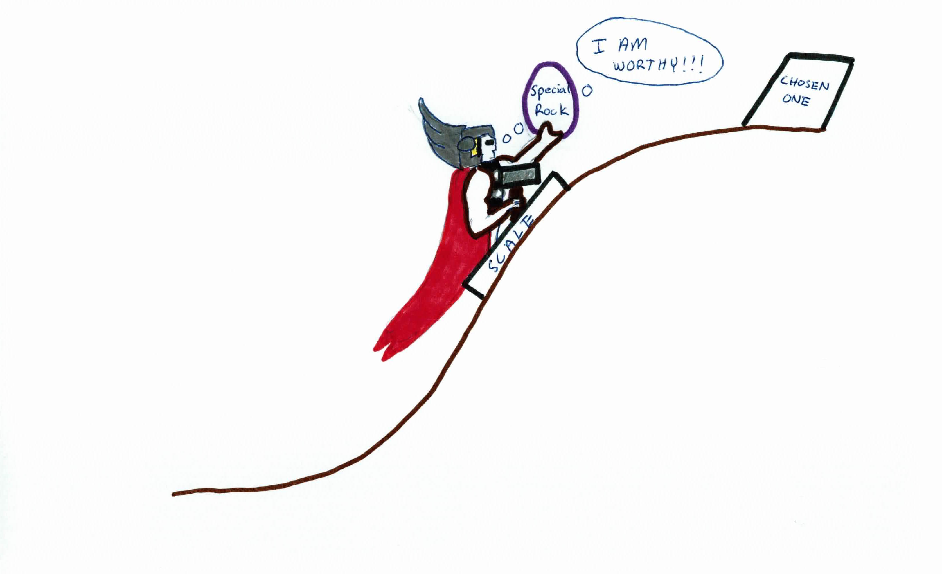
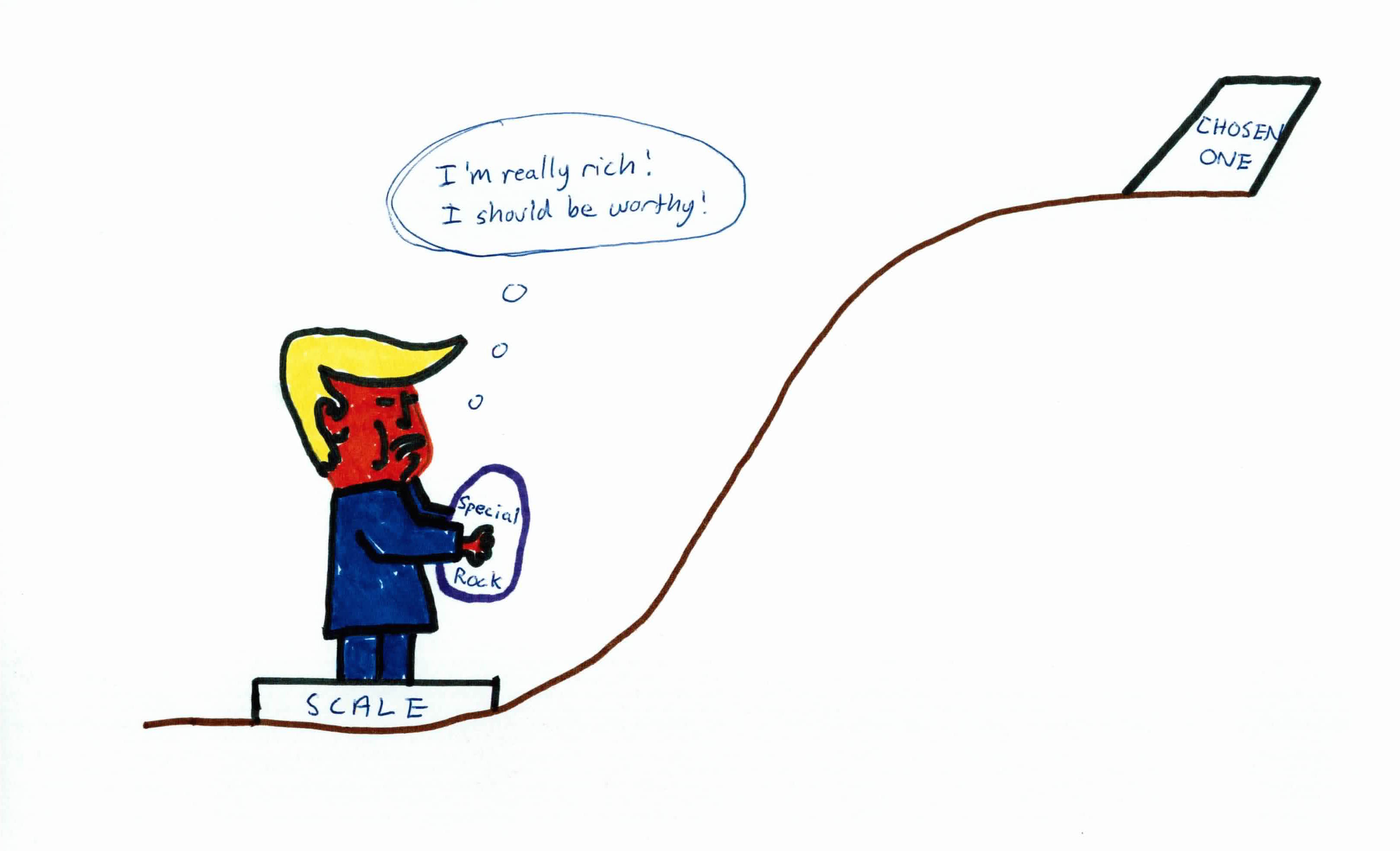
The special hill is near impossible to climb from the start through brute force. So, you implement a special machine with a special rock. The special machine has a scale you step on and acts like an escalator that will move you up the hill. The scale looks for a certain weight, and the closer you are to that weight, the further the machine will take you up the hill.
The special rock is similar to Thor's hammer, in that only people 'worthy' enough can operate it. Over decades the special rock has learned who is 'worthy' and who is not through seeing millions of people try to get to the top. The special rock gets you closer to the weight the more 'worthy' you are. In order for someone to use the machine, a person must step onto the scale on the machine with the special rock.
If the special machine takes someone at least 50% (threshold) up the hill, then you predict that they can make it to the top (positive class), and they're classified as worthy. The higher the machine takes them, the more confident you are that they can make it. If the machine doesn't reach 50%, you assume that they're not going to make it to the top, and are not worthy (negative class). There are some gritty people that could've made it to the top even if the machine goes less than 50%, but we assume they can't if the machine doesn't meet the threshold (misclassification).
Logistic regression is the go-to method for binary classification problems. It's a discriminate model because it estimates the probability $p(y\mid x)$ directly from the training data by minimizing error.
We can't use linear regression because it is extremely sensitive to anomalies and will perform poorly, as some of the predictions will be outside [0,1] and change our threshold. For example, in our plot below, we can see that the threshold for whether we predict if someone is alert or not is near the middle.
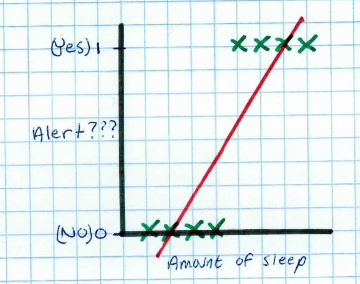
But what happens when we have another piece in our training set that received more sleep? It ends up severely lowering our threshold and ruining our model.
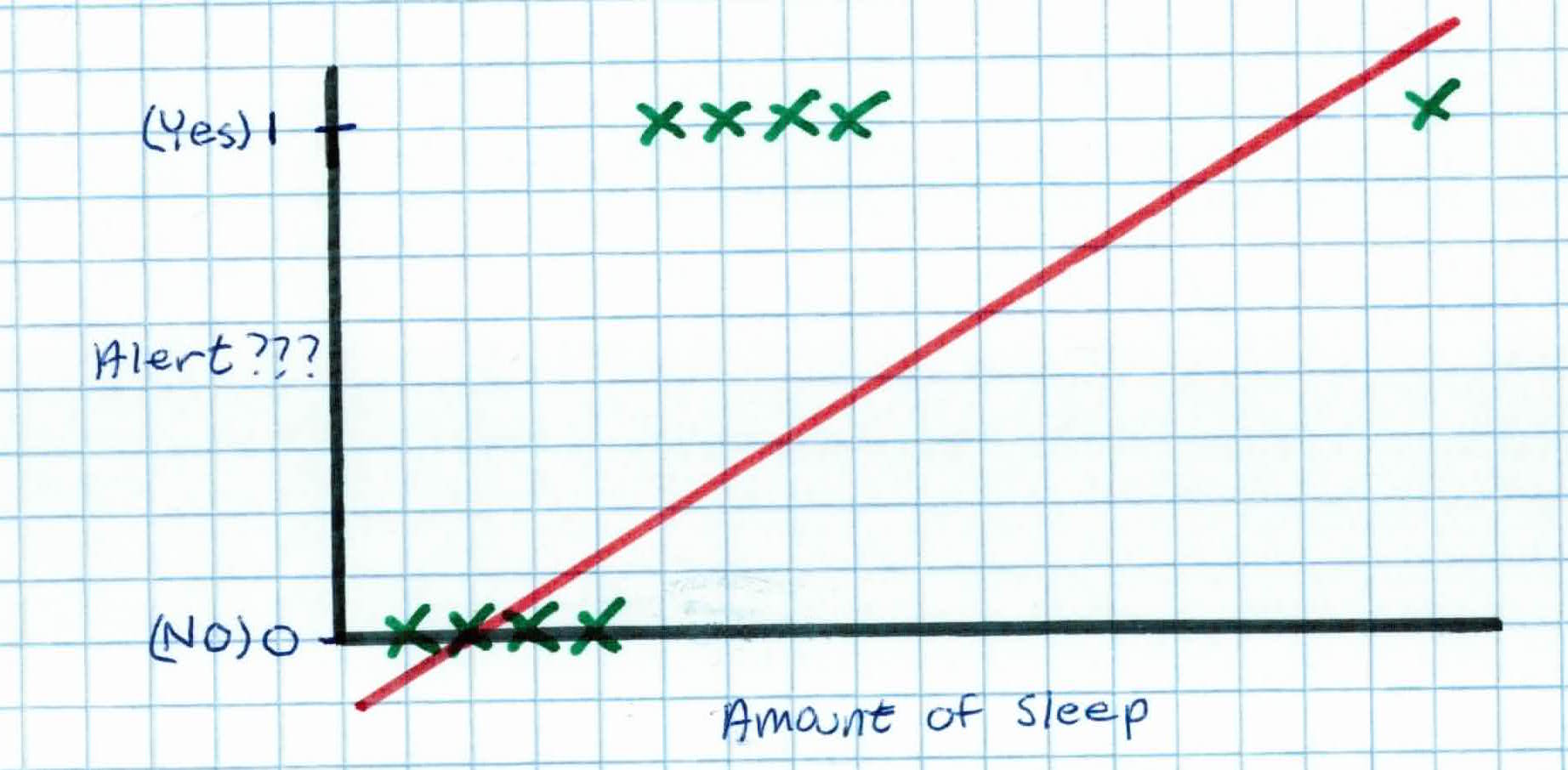
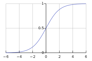
So, logistic regression maps the linear combination of weights and features to a s-shaped function that returns a probability between 0 and 1.
Given $(x_1, y_1), \dots, (x_n, y_n)$ where $x_i \in \mathbb{R}^d$ and $y_i$ is discrete and binary, $y_i \in \mathbb{Y}$ like $\mathbb{Y} = {-1, +1}$ or $ \mathbb{Y} = {0,1}$.
Your task is to learn a classification function: $f: \mathbb{R}^d \rightarrow \mathbb{Y}$. While we want a binary output, we still know we have limitations. For example, we can't predict Credit Card Default with any certainty. But suppose we want to predict how likely is a customer to default, where we output a probability between 0 and 1 that a customer will default. That makes sense and would be suitable and practical. We can then set the threshold to make it binary.
In this case, the output is real (regression) but is bounded (classification) between 0 and 1.
How do we guarantee that $0 \leq f(x) \leq 1$ where $f(x) = p(y=1\mid x)$? We use the sigmoid function:
$$g(z) = \frac{e^z}{1+e^z} = \frac{1}{1+e^{-z}}$$
$$g(z) \rightarrow 1 \ when \ z \rightarrow + \infty $$
$$g(z) \rightarrow 0 \ when \ z \rightarrow - \infty$$
$$g(w_0 + w_1 x) = \frac{1}{1 + e^{-w_0 + w_1 x}}$$
Recall that our function $f(x)=g(w_0 + \sum_{j=1}^dw_j x_j )$ can be written as $f(x) = g(\sum_{j=0}^d w_j x_j)$ if we append 1 to all $x$.
For example, appending 1 to x we get:
$$x = \left(\begin{array}{c} 1 \\ x_1 \\ x_2 \end{array} \right)$$
Taking the dot product of $x$ and $w$ we get:
$$x^T w = \left(\begin{array}{ccc} 1 & x_1 & x_2 \end{array} \right) \left(\begin{array}{c} w_0 \\ w_1 \\ w_2 \end{array} \right) =w_0 + x_1w_1 + x_2 w_2$$
$$=\sum_{j=0}^d w_j x_j$$
Note that outliers won't shift our S-shaped function like it would for linear regression.
In other words, cast the output to bring the linear function quantity between 0 and 1. (Note, one can use other S-shaped functions). If it is above 0.5, we predict 1. Else, we predict 0.
How do we find $w 's$? Just like linear regression, we want to minimize the risk/cost function:
$$J(w) = \frac{1}{n}\sum_{i=1}^n \frac{1}{2}(f(x_n)-y_n)^2$$
Our risk function $J$ makes sense because we are trying to minimize the difference between our prediction and the actual answer (labels).
Remember, $f(x)$ is now the logistic function so the $(f(x)-y)^2$ is not the quadradic function we had when $f$ was linear. Instead, the cost is a complicated non-linear function. Consequently, there are many local optima, hence gradient descent may not find the global optimum.
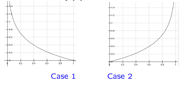
So, we need a different function that is convex. The new convex function is:
$$Cost(f(x), y) = \left \{ \begin{array}{rcl} -log(f(x)) & if \ y=1 \\ -log(1-f(x)) & if \ y=0 \end{array} \right.$$
Putting these functions into one compact function (because $y=0$ or $y=1$):
$$J(w) = -\frac{1}{n}\sum_{i=1}^n y_ilog(f(x_i)) + (1-y_i)log(1-f(x_i))$$
Make sure you understand why the above convex function and its graph works!
Notice that we can derive the same cost function $J$ with a probabilistic interpretation:
$$p(y=1\mid x) = f(x)$$
$$p(y=0\mid x) = 1 - f(x)$$
which can be compactly written as:
$$p(y\mid x) = (f(x))^y(1-f(x))^{1-y}$$
Recall that $(x_1, y_1), \ldots, (x_n, y_n)$ are independently generated. So, the probability of getting $y_1, \ldots, y_n$ in distribution $\mathcal{D}$ from the corresponding $x_1, \ldots, x_n$ is:
$$p(y_1,\ldots, y_n|x_1,\ldots, x_n) = \prod^n_{i=1} p(y_i\mid x_i)$$
This gives us the likelihood of the parameters for $n$ training examples:
$$likelihood(w) = \prod^n_{i=1}p(y_i\mid x_i)$$
$$= \prod^n_{i=1}f(x_i)^{y_i}(1-f(x_i))^{1-y_i}$$
It is easier to work with logs so we take the log of the $likelihood$ function and minimize the negative log likelihood:
$$-log(likelihood(w))$$
$$=-\frac{1}{n}\sum^n_{i=1}y_ilog(f(x_i))+(1-y_i)log(1-f(x_i))$$
which gives us the same cost function as before.
Our goal is to find the right parameter/weights $w$'s to minimize the cost function $J(w)$. To do so, we use gradient descent.
Before talking more, make sure you understand partial derivatives/gradients.
Gradient Descent is an iterative, optimization method that repeats until converge (it has found the minimum). For instance, let's say we have a convex cost function and our goal is to find the $w$ that minimizes it. If we plot it, it looks like so:
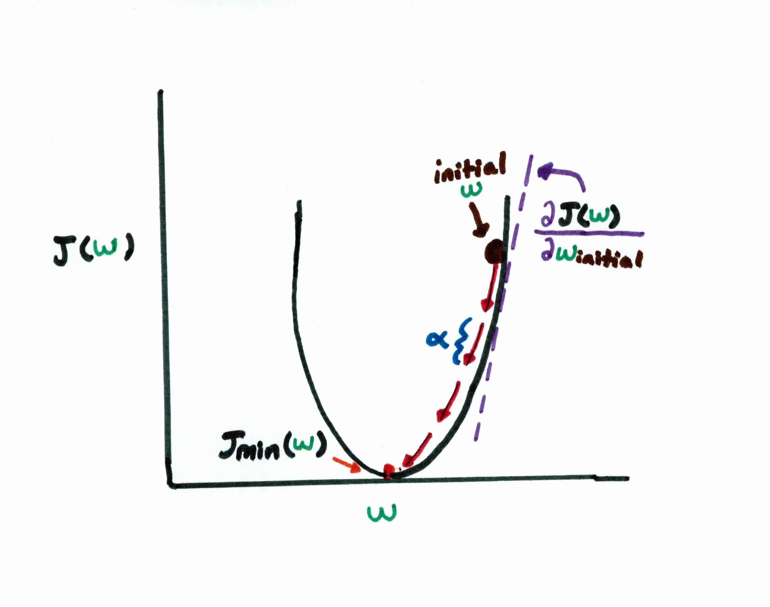
Recall that in gradient descent, we start off by initializing our weights randomly, which puts us at the black dot at the top right on the diagram above. Taking the derivative, we see the slope at this point is a pretty big positive number. We want to move closer to the center, because we want to find the minimum cost, so naturally, we should take a pretty big step $\alpha$ in the opposite direction of the gradient of the function at that point. If we repeat the process enough, we soon find ourselves nearly at the bottom of our curve and much closer to the optimal weight. Convergence means our gradient/slope is at or near zero because this means we found the minimum.
Notice that this only easily happens if our cost function is convex (bowl-shaped), like the cost function in linear regression, because then our descent will always find the global minima. This is why we had to change our cost function earlier to a convex one, because the original one was a complicated non-linear function like so:
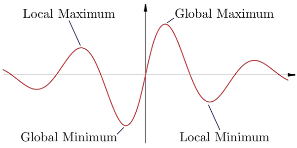
This becomes a problem because we always start by initializing the $w$'s in a random spot, making it possible that gradient descent won't find the global minima and end up in a local minima which represents suboptimal solutions.
So running gradient descent, we repeat until convergence:
After some calculus, we get:
Remember that choosing the right step size $\alpha$ is very important. If the step size is too small, it will take an extremely long time to converge. If it's too large, you'll overshoot the global minimum.
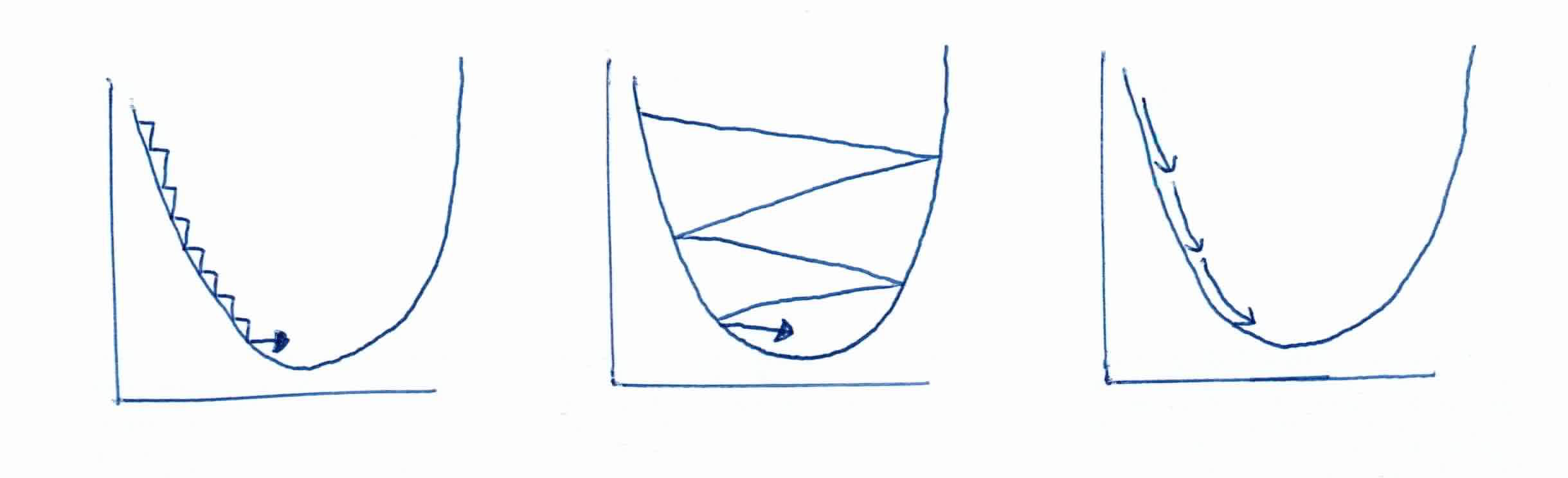 (Left) \(\alpha\) is too small. (Middle) \(\alpha\) is too big. (Right) \(\alpha\) is just right.
With the right $\alpha$, gradient descent will converge, finding the optimal weights.
Note: Gradient descent for logistic regression is the same as linear regression BUT with the new function f(x).
Given a training set ${(x_1, y_1), \ldots (x_n, y_n)}$ with $d$ features, # of iterations $M$, and learning rate $\alpha$ the algorithm for logistic regression works like this:
You're Vegas and you want to predict whether an NBA team will win a ring or not. You're given data on 3 teams, their features, and their label (whether they have won a championship). Their features are number of Hall of Famers, and number of All-Stars, i.e. $x_4 = (7,6)$ means the 4th team has 7 Hall of Famers and 6 All-Stars.
Our learning rate $\alpha$ is set to $0.1$, iterations set to 100, and our training data is given as follows:
$$x_1 = (1,1), y_1 = 0$$
$$x_2 = (4,2), y_2 = 1$$
$$x_3 = (2,4), y_3 = 1$$
Remember that we append a 1 to all our examples so we can also solve for $w_0$. Our updated data is:
$$x_1 = (1,1,1), y_1 = 0$$
$$x_2 = (1,4,2), y_2 = 1$$
$$x_3 = (1,2,4), y_3 = 1$$
First we initialize all $w$'s to zero:
$$w = (0,0,0)$$
Using gradient descent, we look for our betas with the algorithm:
$$w_0 := 0 - 0.1[(0-\frac{1}{2})(1) + (1-\frac{1}{2})(1) + (1-\frac{1}{2})(1)]$$
$$=0 + 0.1[- \frac{1}{2} + 1]$$
$$w_0 =0+ 0.1[\frac{1}{2}] = 0.05$$
Now looking for $w_1$ and $w_2$:
$$w_1 := 0 - 0.1[(0-\frac{1}{2})(1) + (1-\frac{1}{2})(4) + (1-\frac{1}{2})(2)] = .25$$
When we calculate $w_2$ we see that it also comes to .25. So your new $w$ weights are $(.05, .25, .25)$. This is after one iteration.
After 100 iterations, we get:
$$w = \left(\begin{array}{c} -2.707 & .9207 & .9207 \end{array} \right) $$
These weights correctly find a separating line between our positive and negative examples.
For our new example $X_{new} = (3.5, 4)$, with 3.5 Hall of Famers and 4 All-Stars, we want to predict whether this is a championship team. We simply place our features through the sigmoid with our newfound $w$'s:
$$\frac{1}{1+e^{-(-2.707 + (.9207)(3.5) + (.9207)(4))}}$$
$$\frac{1}{1 + e^{-4.2}}$$
$$=.982$$
$.982 > 0.5$, therefore we predict that this team will indeed win a championship!
Logistic regression is a model where the dependent variable is categorical, i.e. 1 or 0, dead or alive, etc. The inputs along with weights are taken and squeezed through a non-linear function such as a sigmoid. This outputs a value between 0 and 1 which corresponds to a probability of how likely the class belongs to it. In order to find the weights you use gradient descent, similar to linear regression.
Other observations: